1. 线性回归

        线性回归中的数学知识

在线性回归中,最重要的莫过于在一大堆的数据中找回归方程

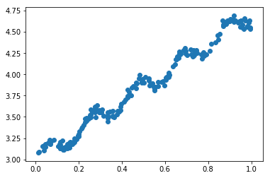
比较简单的方法是,可以利用最小二乘法寻找误差最小的那条直线.

利用最小二乘法计算loss可以写为:

        

为了找到loss最小的那条直线,我们可以对w求导,得到

        

        

因此求回归方程转变为求参数w.

        实现代码

def standRegres(xArr,yArr):     xMat=np.mat(xArr)     yMat=np.mat(yArr).T     xTx=xMat.T*xMat     if np.linalg.det(xTx)==0.0:         print('error')         return     ws=xTx.I*(xMat.T*yMat)     return ws

求出参数w

        将回归直线去拟合实际数据

import matplotlib.pyplot as plt fig=plt.figure() ax=fig.add_subplot(111) ax.scatter(xMat[:,1].flatten().A[0],yMat.T[:,0].flatten().A[0]) xCopy=xMat.copy() xCopy.sort(0) yHat=xCopy*ws ax.plot(xCopy[:,1],yHat) plt.show()

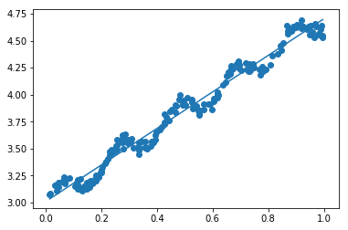
可以看到虽然直线显示了大概的趋势,但并不能很好的去拟合数据,下面介绍一种强大的回归--""局部加权线性回归"",可解决上面这个拟合度不够的问题.

    2. 局部加权线性回归

        局部加权线性回归中的数学知识

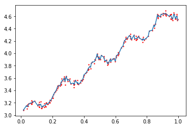
相对于线性回归 , 局部加权的意思是对于每一个特征 , 都给添加一个权重 , 然后基于普通的最小均方差来进行回归.

这里使用高斯核进行计算每一个点的权重

        

对于w^的计算和上面类似,只是添加了权重w

        

        实现代码

def lwlr(testPoint,xArr,yArr,k=1.0):     xMat=np.mat(xArr)     yMat=np.mat(yArr).T     m=np.shape(xMat)[0]     weights=np.mat(np.eye((m)))     for j in range(m):         diffMat=testPoint-xMat[j,:]         weights[j,j]=np.exp(diffMat*diffMat.T/(-2.0*k**2))     xTx=xMat.T*(weights*xMat)     if np.linalg.det(xTx)==0.0:         print("error")         return     ws=xTx.I*(xMat.T*(weights*yMat))     return testPoint*ws def lwlrTest(testArr,xArr,yArr,k=1.0):     m=np.shape(testArr)[0]     yHat=np.zeros(m)     for i in range(m):         yHat[i]=lwlr(testArr[i],xArr,yArr,k)     return yHat

        拟合效果

    

import matplotlib.pyplot as plt fig=plt.figure() ax=fig.add_subplot(111) ax.plot(xSort[:,1],yHat[srtInd]) ax.scatter(xMat[:,1].flatten().A[0],np.mat(yArr).T.flatten().A[0],s=2,c='red') plt.show()

代码和数据均已上传到,有需要的朋友可以下载..

GitHub

码云